Invest Smarter: From Triangles to Polygons

From Triangles to Polygons: A Smarter Approach to Investing

From Triangles to Polygons: A Smarter Approach to Investing

Investing is like building a 3D puzzle. Traditionally, portfolios are built piece by piece, using small, individual investments like stocks or bonds. This is similar to constructing a surface using only triangles—a reliable but sometimes inefficient approach. What if we could use larger, more flexible shapes like polygons (squares, hexagons, etc.) to simplify and improve the structure? By applying this metaphor to investing, we can create diversified, efficient, and adaptable portfolios.

From Triangles to Polygons in Investing

  1. Triangles: These represent individual investments like a single stock or bond. They are simple and easy to manage but often require many pieces to build a stable portfolio.
  2. Polygons: These represent broader investments, such as ETFs, mutual funds, or diversified portfolios. Using polygons allows for better coverage with fewer pieces, reducing complexity while improving efficiency.

Moving from triangles to polygons in investing means transitioning from managing many small, standalone investments to grouping assets into more comprehensive and diversified categories.

How It Works in Practice

  1. Portfolio Diversification: Adding a mix of assets (stocks, bonds, real estate, crypto) is like replacing many small triangles with larger polygons. It provides broader market exposure with less effort.
  2. Risk Management: Just as polygons smooth a surface, diversification smooths portfolio performance by reducing the impact of any one investment.
  3. Efficiency: Instead of managing dozens of individual stocks, using an ETF or mutual fund simplifies the process, much like using fewer polygons to model a 3D surface.
  4. Adaptability: Markets change over time. Rebalancing your portfolio is like reshaping polygons to fit a new model, ensuring your investments align with your goals and market conditions.
  5. Cutting and Joining: Selling underperforming investments (cutting) and adding promising ones (joining) refines your portfolio, making it more effective—just like improving a polyhedral surface.

Why It Matters

  • Better Returns: Diversification and risk management help smooth out volatility and provide steadier returns.
  • Simplified Management: Grouping investments into funds or portfolios reduces the complexity of managing individual assets.
  • Resilience: A well-structured portfolio can better withstand market downturns, just as a stable polyhedral surface handles stress.
  • Efficiency: Fewer investments with broader coverage save time and reduce costs, similar to modeling with fewer, larger polygons.

An Everyday Example

Think about building a soccer ball. A soccer ball isn’t made of triangles—it uses hexagons and pentagons to create a smooth, round shape with fewer pieces. In investing, this is like using diversified funds (ETFs or mutual funds) instead of many individual stocks. It’s simpler, more efficient, and creates a better-rounded portfolio.

A Smarter Approach to Investing

Moving from “triangles” to “polygons” in your investment strategy helps you build a portfolio that’s diversified, efficient, and adaptable. By embracing these principles, you can create a financial plan that’s better equipped to handle market fluctuations and achieve your goals.

Upgrade Your 3D Models: From Triangles to Polygons

From Triangles to Polygons: A Better Way to Build 3D Models

From Triangles to Polygons: A Better Way to Build 3D Models

Imagine you’re working on a jigsaw puzzle. Traditionally, you’ve only used triangular pieces to complete the picture. Triangles are simple to work with, but what if you could use a mix of shapes—like squares or pentagons? That’s exactly the idea behind moving from triangulations to polyhedral surfaces. This upgrade allows us to create better, more efficient 3D models and designs with fewer pieces.

What Are Triangles and Polygons?

– **Triangles**: These are simple, stable shapes. Any surface can be broken down into triangles, which makes them reliable for 3D modeling. However, using only triangles often requires a lot of them to create smooth and detailed designs.
– **Polygons**: These are shapes with more sides, like squares, pentagons, or hexagons. Using polygons allows us to build complex surfaces more efficiently, with fewer pieces while still keeping the design smooth and accurate.

How It Works

  1. Triangles vs. Polygons: Instead of relying only on triangles, we introduce polygons as building blocks. This adds flexibility and reduces the number of pieces needed for a design.
  2. Updating the Rules: Just like you might change the rules of a game for new players, we update the mathematical definitions and tools to handle polygons instead of just triangles.
  3. Making Surfaces Smoother: Imagine ironing out a crumpled sheet. Using larger polygonal pieces (instead of lots of small triangles) makes it easier to smooth out surfaces with fewer steps.

Why It’s Useful

  • Better 3D Models: Using polygons helps create detailed models for video games, movies, or 3D printing without requiring as much computing power.
  • Cool Architecture: Architects use polyhedral surfaces to design intricate structures, like domes or curved walls, with fewer pieces and greater creativity.
  • Medical Imaging: Doctors can create more accurate 3D models of body parts, like bones or organs, using polyhedral surfaces.
  • Engineering Simulations: Engineers use these surfaces to test how structures like bridges or cars handle stress and pressure.
  • Biological Models: Polyhedral surfaces can even represent complex biological systems, like the structure of proteins or cells.

An Everyday Example

Think about a soccer ball. It’s made up of hexagons (six-sided shapes) and pentagons (five-sided shapes). If you tried to make it using only triangles, you’d need a lot more pieces to make it look round. Using hexagons and pentagons allows for a smoother and more realistic design with fewer pieces. That’s the power of polyhedral surfaces!

Why It’s Exciting

Moving from triangles to polygons is like upgrading your toolbox. You get more options to create amazing designs, whether it’s for movies, buildings, or scientific research. It’s not just about making things look better—it’s also about working smarter and solving problems more efficiently.

Investing Strategies Inspired by 3D Mesh Theory

Investing Lessons from 3D Mesh Theory

Investing Lessons from 3D Mesh Theory

What do investing and 3D modeling have in common? Quite a lot, if you think of investing as building a strong, adaptable structure—much like creating 3D models with triangle meshes. The concept of discretely equivalent triangle meshes teaches us how to modify structures while keeping their overall shape intact. By applying this metaphor, we can explore smarter ways to manage portfolios and make investment decisions.

Extensions: Investing Like a 3D Puzzle

  1. Smoothing the Portfolio: Diversifying your investments is like adding more, smaller triangles to a mesh to smooth out rough edges. A balanced portfolio reduces risk and ensures steady growth.
  2. Using Different Shapes: Instead of relying solely on one asset type (e.g., stocks), include a mix like bonds, ETFs, real estate, or cryptocurrencies. This diversification helps your portfolio adapt to market changes.
  3. Adjusting for Market Curves: Markets rise and fall like curved surfaces. Strategies like rebalancing and dollar-cost averaging help you navigate these ups and downs.
  4. Dynamic Adjustments: Just as meshes can be dynamically adjusted, you can shift your investments based on changing market conditions, reallocating to growth sectors or safer options as needed.
  5. Cutting and Joining: Selling underperforming assets (cutting) or investing in promising opportunities (joining) reshapes your portfolio for better performance.

Applications: Real-World Investment Strategies

  • Making Investing Smoother: Regular contributions to your portfolio, like dollar-cost averaging, smooth out returns over time.
  • Saving Time and Effort: Simplify your portfolio with index funds or ETFs that mimic the market, much like optimizing a mesh for efficiency.
  • Stress Testing: Financial stress testing shows how your portfolio would perform in tough conditions, just as engineers test the strength of structures.
  • Helping Financial Planning: Advisors use models of your wealth to help plan for goals like retirement, similar to doctors using 3D meshes for surgeries.
  • Balancing Risk and Reward: Rebalancing your portfolio ensures you maintain the right mix of assets, balancing growth and safety like a stable mesh structure.
  • Navigating Markets: Just as robots use 3D meshes to navigate spaces, investors use analysis tools to navigate financial markets.
  • Understanding Complex Products: Visualizing your portfolio like a 3D structure makes it easier to grasp financial products and their roles.
  • Continuous Learning: Monitoring and tweaking your portfolio over time helps you learn what works, much like refining a 3D model for better results.

Why It’s Cool in Investing

The theory of discretely equivalent triangle meshes teaches us the value of adaptability, diversification, and continuous improvement. In investing, these same principles help us reduce risks, smooth out returns, and adapt to market fluctuations. Whether you’re saving for retirement or building wealth, thinking like a 3D puzzle master can help you craft a portfolio that’s both stable and flexible.

Mastering Discretely Equivalent Triangle Meshes

Understanding Discretely Equivalent Triangle Meshes

Understanding Discretely Equivalent Triangle Meshes

Imagine a triangle mesh as a 3D puzzle made of tiny triangles. These meshes are used to create 3D models for things like video game characters, animations, or even 3D-printed objects. The concept of discretely equivalent triangle meshes focuses on modifying these puzzles while keeping their overall shape and structure the same. Let’s explore how this theory can be extended and applied in the real world.

Extensions: Making the Puzzle Even Better

  1. Smoothing the Puzzle: Adding more, smaller triangles makes rough surfaces look smoother, similar to upgrading a pixelated image to high resolution.
  2. Using Different Shapes: Replacing triangles with other shapes, like squares, allows for more flexibility in creating models.
  3. Curves and Bumps: Adjusting triangles to fit curved surfaces, like a ball or a human face, enhances realism.
  4. Stretchy or Moving Puzzles: Allowing triangles to move or stretch helps animate characters or simulate materials like rubber.
  5. Cutting and Gluing: Cutting apart or joining puzzle pieces makes it possible to design complex objects with moving parts or hollow areas.

Applications: How It’s Used

  • Movies and Games: 3D characters in movies or games are created using triangle meshes. Keeping them equivalent ensures smooth animations and effects.
  • Saving Time and Effort: Designers simplify models while maintaining detail, making rendering faster and easier.
  • Engineering and Safety Testing: Engineers use triangle meshes to test how structures handle stress, ensuring accurate results.
  • Helping Doctors: 3D models of organs help doctors plan surgeries or study diseases.
  • 3D Printing: Equivalent meshes ensure that digital designs match the printed objects.
  • Robotics and Drones: Robots use 3D meshes to understand and navigate their surroundings.
  • Studying Nature: Scientists model proteins or cells to learn more about biology and medicine.
  • Math Made Fun: Mathematicians use these meshes to visualize complex ideas in geometry.

Why It’s Cool

The theory of discretely equivalent triangle meshes is like a toolbox for working with 3D puzzles. It powers many of the amazing things we see in movies, games, and technology, making processes faster, more accurate, and creative. Whether it’s helping doctors, animators, or engineers, this theory proves how 3D puzzles can solve real-world challenges.

Dynamic Modeling of CAR T Cells: A Financial Approach

Applying Financial Lattice Models to CAR T Cell Therapy

Applying Financial Lattice Models to CAR T Cell Therapy

The principles of financial lattice models, optimization, and forecasting can be effectively applied to CAR T cell therapy, a groundbreaking approach in cancer treatment. By leveraging concepts like action minimization, dynamic forecasting, and multidimensional analysis, researchers and clinicians can enhance the efficiency and predictability of CAR T cell therapies.

1. Conceptual Mapping: From Finance to CAR T Cells

Financial Model Concept CAR T Cell Application
Lattice Framework (N, M, K) Time steps (N), cell types (M), and treatment conditions (K).
Prices and Volatility CAR T cell concentrations, tumor load, cytokine levels, or patient biomarkers.
Action Minimization Optimizing CAR T cell dosages or schedules to minimize tumor load while controlling cytokine storms.
Forecasting Predicting tumor response or CAR T cell expansion and persistence over time.
Portfolio Optimization Balancing therapeutic effectiveness with toxicity risks.

2. Tumor-CAR T Cell Dynamics

The interaction between CAR T cells and tumor cells can be modeled using discrete dynamical equations. For example:

    Tn+1 = Tn - k1 * Tn * Cn
    Cn+1 = Cn + k2 * Cn * (1 - Cn/Cmax) - k3 * Tn * Cn
    

Here, T represents tumor load, C is the CAR T cell concentration, and the coefficients (k1, k2, k3) control interaction dynamics.

3. Lattice Simulation Code

    import numpy as np
    import matplotlib.pyplot as plt

    # Parameters
    N = 30  # Time steps (days)
    T0 = 1e6  # Initial tumor load (cells)
    C0 = 1e5  # Initial CAR T cell concentration (cells)
    k1, k2, k3 = 1e-8, 0.1, 1e-8  # Interaction coefficients

    # Initialize tumor and CAR T cell dynamics
    tumor = np.zeros(N)
    cart = np.zeros(N)
    tumor[0], cart[0] = T0, C0

    # Dynamics simulation
    for n in range(1, N):
        tumor[n] = tumor[n-1] - k1 * tumor[n-1] * cart[n-1]
        cart[n] = cart[n-1] + k2 * cart[n-1] * (1 - cart[n-1] / (1e6)) - k3 * tumor[n-1] * cart[n-1]

    # Visualization
    plt.figure(figsize=(10, 6))
    plt.plot(range(N), tumor, label="Tumor Load", color="red")
    plt.plot(range(N), cart, label="CAR T Cells", color="blue")
    plt.title("Tumor and CAR T Cell Dynamics")
    plt.xlabel("Time (days)")
    plt.ylabel("Cell Count")
    plt.legend()
    plt.grid()
    plt.show()
    

4. Forecasting and Optimization

Forecasting tumor regression or CAR T cell persistence helps predict treatment outcomes. The following Python code illustrates the concept:

    from sklearn.linear_model import LinearRegression

    # Forecast tumor response
    X = np.arange(N).reshape(-1, 1)  # Time steps
    y = tumor.reshape(-1, 1)         # Tumor load
    model = LinearRegression()
    model.fit(X, y)
    forecast = model.predict(np.arange(N, N + 10).reshape(-1, 1))
    

This technique can be extended using machine learning models like LSTMs for more complex predictions.

5. Conclusion

Applying financial lattice models to CAR T cell therapy provides a structured way to model dynamics, optimize treatments, and forecast outcomes. These techniques hold promise for improving the efficacy and safety of CAR T cell therapies in clinical settings.

How to Optimize Investment Portfolios Using Lattice Dynamics

Optimizing Financial Markets with Lattice Dynamics

Optimizing Financial Markets with Lattice Dynamics

Learn how to apply mathematical modeling for portfolio optimization, trend forecasting, and real-time market analysis.

What Are Lattice Dynamics?

Lattice dynamics is a mathematical framework originally used in physics to model systems like crystals and waves. In finance, we can use a similar approach to model the interactions of multiple financial metrics, such as stock prices, volatility, and market conditions, over time.

Imagine a 3D grid where each point represents the price of an asset (like Apple or Tesla) at a specific time under certain market conditions. By analyzing these points and their relationships, we can uncover trends, optimize portfolios, and even predict future price movements.

How It Works

Our model uses a mathematical tool called a pluri-Lagrangian formulation to study changes in stock prices and their volatility. Here’s the process:

  1. Fetch Real Market Data: We use historical stock prices from platforms like Yahoo Finance.
  2. Build a Lattice: The data is organized into a 3D grid, where each dimension represents time, different assets, and market conditions (like volatility).
  3. Optimize Trends: The model minimizes sudden changes or inconsistencies in price trends, creating a smoother and more predictable representation.
  4. Forecast Future Prices: Using the optimized trends, we predict where prices might go in the next few days or weeks.
  5. Optimize Portfolios: By balancing returns and volatility, we calculate the best allocation of investments across multiple assets.

Code in Action

Here’s a simplified explanation of how the code works:

  • Fetch historical stock data using Python and the Yahoo Finance API.
  • Build a “lattice” by organizing stock prices and volatility into a 3D matrix.
  • Apply mathematical equations to smooth the trends and identify patterns.
  • Visualize the results using graphs, showing optimized trends and future forecasts.

The code is designed to handle multiple assets and provides outputs such as optimized price trends, portfolio weights, and forecasted prices.

Visual Outputs

The model generates the following visualizations:

1. Initial Price Trends

2. Optimized Price Trends

optimized

3. Portfolio Trends

portfolio

4. Forecasted Prices

Forecasted Prices

Time Step AAPL MSFT GOOGL AMZN TSLA
1 242.23 434.73 175.80 210.94 361.28
2 243.24 435.25 175.26 210.61 363.46
3 244.25 435.77 174.71 210.28 365.63
4 245.25 436.29 174.16 209.95 367.81
5 246.26 436.81 173.62 209.62 369.99

What You Can Learn

This model helps investors answer questions like:

  • How are stock prices likely to behave over time?
  • Which assets should I invest in to minimize risk and maximize returns?
  • Can I predict future price movements with historical trends?

Conclusion

The integration of mathematical modeling and financial data provides a powerful tool for understanding and optimizing market behavior. Whether you’re a seasoned investor or just starting, these techniques can help you make more informed decisions.

Want to try it out? Download the code and see the results for yourself!

import numpy as np
import pandas as pd
import yfinance as yf
import matplotlib.pyplot as plt
import time

# Financial lattice dimensions
N = 20  # Time steps
M = 5   # Number of assets
K = 2   # Market condition (prices + volatility)

# Fetch market data
def fetch_market_data(tickers, period="1mo", interval="1d"):
    data = {}
    for ticker in tickers:
        df = yf.download(ticker, period=period, interval=interval)
        data[ticker] = df['Close'].values[:N]  # Use only first N time steps
    return np.array(list(data.values())).T  # Transpose to align with lattice

# Compute rolling volatility as a new dimension
def compute_volatility(prices, window=5):
    return np.array([np.std(prices[max(0, i - window):i+1], axis=0) for i in range(prices.shape[0])])

# Extend lattice with volatility
def extend_with_volatility(prices):
    volatility = compute_volatility(prices[:, :, 0])
    volatility = volatility.reshape(prices.shape[0], prices.shape[1], 1)  # Match dimensions
    return np.concatenate([prices, volatility], axis=2)

# Lagrangian densities for price differences
def L_nm(price_nm, price_n1m, epsilon=1e-8):
    diff = price_n1m - price_nm
    return np.log(np.maximum(diff, epsilon))

# Variational action minimization
def minimize_action(prices, iterations, epsilon=1e-8, tolerance=1e-6):
    N, M, K = prices.shape
    for step in range(iterations):
        new_prices = prices.copy()
        for n in range(1, N - 1):
            for m in range(1, M - 1):
                for k in range(K):  # Prices and volatility
                    action_nm = L_nm(prices[n, m, k], prices[n+1, m, k], epsilon)
                    total_action = action_nm
                    
                    # Update prices using gradient descent
                    new_prices[n, m, k] = np.clip(prices[n, m, k] - 0.01 * total_action, 0, np.max(prices))
        
        # Check convergence
        max_change = np.max(np.abs(new_prices - prices))
        if max_change < tolerance:
            print(f"Converged at step {step} with max change {max_change:.8f}")
            break
        prices = new_prices
    return prices

# Forecast prices based on optimized trends
def forecast_prices(prices_optimized, steps=5):
    N, M, K = prices_optimized.shape
    forecasts = []
    for m in range(M):
        x = np.arange(N)
        y = prices_optimized[:, m, 0]  # Optimized price trends
        coefficients = np.polyfit(x, y, deg=1)  # Linear fit
        forecast = np.polyval(coefficients, np.arange(N, N + steps))
        forecasts.append(forecast)
    return np.array(forecasts).T  # Transpose to align time steps

# Portfolio optimization: minimize volatility
def optimize_portfolio(prices):
    returns = np.diff(prices[:, :, 0], axis=0)  # Compute returns from prices
    avg_returns = np.mean(returns, axis=0)
    volatility = np.std(returns, axis=0)

    # Minimize volatility while maintaining return > threshold
    threshold = 0.01  # Minimum return
    weights = np.zeros(prices.shape[1])  # Initialize weights
    for m in range(prices.shape[1]):
        if avg_returns[m] > threshold:
            weights[m] = 1 / volatility[m]
    weights /= np.sum(weights)  # Normalize weights
    return weights

# Apply weights to compute optimized portfolio trend
def compute_portfolio_trend(prices, weights):
    portfolio_trend = np.dot(prices[:, :, 0], weights)
    return portfolio_trend

# Plot asset trends
def plot_asset_trends(prices, tickers, title="Price Trends for Selected Assets"):
    plt.figure(figsize=(10, 6))
    for m, ticker in enumerate(tickers):
        plt.plot(prices[:, m, 0], label=f"{ticker}")
    plt.title(title)
    plt.xlabel("Time Steps")
    plt.ylabel("Price")
    plt.legend()
    plt.grid()
    plt.show()

# Plot portfolio trend
def plot_portfolio_trend(portfolio_trend, title="Optimized Portfolio Trend"):
    plt.figure(figsize=(10, 6))
    plt.plot(portfolio_trend, label="Portfolio Trend", color="green")
    plt.title(title)
    plt.xlabel("Time Steps")
    plt.ylabel("Portfolio Value")
    plt.legend()
    plt.grid()
    plt.show()


# Main program
def main():
    # Define tickers for stocks or cryptocurrencies
    tickers = ["AAPL", "MSFT", "GOOGL", "AMZN", "TSLA"]  # Example stocks
    
    # Fetch market data and build initial financial lattice
    market_data = fetch_market_data(tickers, period="1mo", interval="1d")
    prices = market_data.reshape(N, M, 1)  # Initial lattice with prices only
    prices = extend_with_volatility(prices)  # Add volatility as a new dimension
    
    # Plot initial price trends
    plot_asset_trends(prices, tickers, title="Initial Price Trends")
    
    # Minimize action to smooth prices or optimize trends
    iterations = 100
    prices_optimized = minimize_action(prices, iterations)
    
    # Plot optimized trends
    plot_asset_trends(prices_optimized, tickers, title="Optimized Price Trends")
    
    # Portfolio optimization
    weights = optimize_portfolio(prices)
    print(f"Optimized Portfolio Weights: {weights}")
    portfolio_trend = compute_portfolio_trend(prices, weights)
    plot_portfolio_trend(portfolio_trend)
    
    # Forecast future prices
    forecasts = forecast_prices(prices_optimized, steps=5)
    print(f"Forecasted Prices: {forecasts}")

# Run the program
if __name__ == "__main__":
    main()

Understanding Market Dynamics through the Discrete KdV Equation

Investment Insights from the Variational Interpretation of the Discrete KdV Equation

Investment Insights from the Variational Interpretation of the Discrete KdV Equation

How wave dynamics and energy minimization in discrete systems relate to market behavior and portfolio optimization

What is the Discrete KdV Equation?

The Korteweg-de Vries (KdV) equation is a mathematical model used to describe wave dynamics, such as water waves or sound waves. Its discrete form applies to systems with distinct points, like steps on a staircase or data points in financial markets. In investing, this can represent price changes over time, where each point corresponds to market data at a specific moment.

Variational Principles and Investing

The variational principle explains how systems evolve to minimize or optimize certain quantities, such as energy. In investing, this is analogous to:

  • Risk Minimization: Investors aim to reduce portfolio risk while maintaining expected returns, similar to how waves evolve to balance energy.
  • Market Dynamics: Just as wave systems evolve to minimize energy, financial markets exhibit patterns as they balance forces like supply, demand, and volatility.

Why This Matters for Investors

Understanding the variational interpretation of the discrete KdV equation can provide investors with insights into:

  • Market Patterns: The equation explains how trends and cycles (like bullish or bearish markets) emerge as the market seeks equilibrium.
  • Portfolio Optimization: Similar to minimizing energy in wave systems, investors use optimization strategies to balance risk and return in their portfolios.

Applications in Financial Systems

The principles of the discrete KdV equation can be applied to various aspects of investing:

  • Market Trends: Price waves in financial markets can be modeled as discrete wave systems, revealing patterns like cycles and mean reversion.
  • Risk Management: Variational principles guide strategies to minimize portfolio volatility, akin to stabilizing wave systems.
  • Algorithmic Trading: Trading algorithms use optimization techniques inspired by variational methods to predict and capitalize on market movements.

Solitons and Market Stability

One of the most fascinating aspects of the discrete KdV equation is its ability to describe solitons—stable, localized wave patterns. In financial markets, solitons can represent:

  • Persistent Trends: Stable market trends, like long-term growth in an index or a sustained bull market.
  • Market Resilience: Solitons show how systems can maintain stability despite external disturbances, similar to markets recovering after a shock.

Computational Applications in Investing

Just as the discrete KdV equation is used in physics to model waves, its variational principles inspire computational techniques in investing:

  • Portfolio Optimization Algorithms: Techniques derived from variational methods help allocate assets to maximize returns while minimizing risk.
  • Market Simulation: Simulations based on wave dynamics predict market behavior and test trading strategies.
  • Risk Management Models: Variational principles ensure stability in risk assessments over time.

Conclusion

The variational interpretation of the discrete KdV equation provides a powerful framework for understanding both physical systems and financial markets. For investors, it offers:

  • Insights into Market Dynamics: Understanding how price waves form and evolve can guide better decision-making.
  • Tools for Risk Management: Optimization techniques rooted in variational principles can help create stable, resilient portfolios.
  • Applications in Algorithmic Trading: Variational methods inspire sophisticated algorithms to capitalize on market patterns.

By connecting wave dynamics to investing, the discrete KdV equation bridges the gap between mathematical theory and practical financial strategies.

© 2024 | Investing with Mathematical Insights

Applications of Discrete KdV Equation in Real-World Problems

Variational Interpretation of the Discrete KdV Equation

The Variational Interpretation of the Discrete KdV Equation

A detailed exploration of wave dynamics, solitons, and energy minimization in discrete systems

What is the Discrete KdV Equation?

The Korteweg-de Vries (KdV) equation is a mathematical model describing wave dynamics in various physical systems, such as shallow water waves or sound waves. In its discrete form, the equation governs the evolution of waves in systems with distinct, separate points, like beads on a string or steps in a staircase.

What is Variational Interpretation?

The variational principle is a guiding rule in physics and mathematics that systems tend to evolve by minimizing certain quantities, like energy or action. For example:

  • A soap bubble minimizes surface tension to form a perfect sphere.
  • A ball rolls downhill by minimizing its potential energy.

In the discrete KdV equation, the system evolves by minimizing a mathematical functional, which represents the “energy” of the wave system.

Why Does This Matter?

The variational interpretation gives us deeper insights into:

  • Wave behavior: Explains why waves evolve in specific patterns.
  • Energy optimization: Describes how discrete points balance energy while maintaining wave structures.

Applications of the Discrete KdV Equation

The discrete KdV equation is applied in many fields:

  • Lattice Vibrations: Models vibrations of atoms in a crystal lattice.
  • Traffic Flow: Describes waves of congestion in traffic systems.
  • Water Waves: Governs wave dynamics in shallow water with discrete steps.
  • Optical Systems: Explains light pulses in fiber optic networks.

Deriving the Discrete KdV Equation

The discrete KdV equation is derived from the variational principle:

  1. Define the Functional: A mathematical expression represents the system’s energy or action, depending on the positions and interactions of discrete points.
  2. Minimize the Functional: The system evolves by minimizing this energy, leading to a mathematical condition.
  3. Result: This condition gives rise to the discrete KdV equation, which describes how wave points interact and evolve over time.

Solitons and Stability

The discrete KdV equation is famous for describing solitons, stable wave packets that maintain their shape as they travel:

  • Energy Balance: Solitons arise when wave spreading (dispersion) and wave focusing (nonlinearity) balance.
  • Stability: Solitons correspond to energy-minimizing configurations, ensuring their shape remains intact during interactions.

Computational Applications

In computational science, the variational framework is used to:

  • Ensure Stability: Variational methods prevent numerical errors in simulations.
  • Improve Efficiency: Models wave behavior with accurate and computationally efficient algorithms.
  • Simulate Real-World Systems: Models light propagation in fibers, lattice dynamics, and more.

Conclusion

The discrete KdV equation is a cornerstone in understanding discrete systems and wave phenomena. Its variational interpretation offers:

  • Unified Framework: Explains wave behavior across various systems.
  • Practical Tools: Models solitons, stability, and wave evolution.
  • Real-World Applications: From traffic flow to fiber optics and beyond.

The discrete KdV equation connects the elegance of mathematical theory with practical solutions to real-world problems.

Lagrangian Structure in Integrable Hierarchies Explained

Understanding the Lagrangian Structure of Integrable Hierarchies in Simple Terms

Understanding the Lagrangian Structure of Integrable Hierarchies in Simple Terms

The **Lagrangian structure of integrable hierarchies** might sound complex, but it’s a powerful framework for solving dynamic problems. This article explains these concepts in simple terms and shows how they apply to real-life situations like investing or managing complex systems.

What is a Lagrangian?

Imagine you’re driving a car and want to reach your destination as efficiently as possible. You face a trade-off:

  • **Driving fast** gets you there quickly but burns more fuel and may be unsafe.
  • **Driving slowly** saves fuel but wastes time.

The **Lagrangian** is a mathematical way to balance these trade-offs. In physics, it combines:

  • **Kinetic energy**: Effort or motion (like fuel consumption).
  • **Potential energy**: Stored effort (like safety or efficiency).

It helps determine the “best path” to achieve a goal while balancing competing factors.

What Are Integrable Systems?

An **integrable system** is like a perfectly tuned machine where everything moves predictably and harmoniously. These systems have:

  • **Conserved quantities**: Things that don’t change over time, like the total energy in a frictionless pendulum.
  • **Symmetry**: Patterns or rules that stay consistent, making the system easier to analyze.

Think of a train system with a fixed schedule and reliable operations—this is a real-world analogy of an integrable system.

What is a Hierarchy?

A **hierarchy** organizes tasks into levels:

  • **Top level**: Broad, long-term decisions.
  • **Middle level**: Medium-term strategies.
  • **Bottom level**: Specific, short-term tasks.

For example, in investing:

  • **Long-term**: Your retirement savings plan.
  • **Medium-term**: Quarterly portfolio rebalancing.
  • **Short-term**: Daily stock or crypto trades.

The Lagrangian Structure of Integrable Hierarchies

Combining these ideas:

  • The **Lagrangian structure** helps find the “best strategy” for balancing trade-offs.
  • An **integrable hierarchy** ensures that all levels of a system work together harmoniously.

This framework solves dynamic problems by:

  1. Defining trade-offs (e.g., speed vs. fuel efficiency, risk vs. return).
  2. Optimizing for a goal (e.g., fastest route, best investment performance).
  3. Ensuring harmony between different layers of decision-making.

Practical Example: Investing

Let’s apply this to managing an investment portfolio. Imagine you want to balance:

  • **Returns**: Maximizing your gains.
  • **Risk**: Minimizing the chance of losses.

The Lagrangian structure helps solve this by:

  1. **Defining the trade-offs**: Returns are like potential energy (your goal), while risk is like kinetic energy (effort or uncertainty).
  2. **Finding the optimal strategy**: Use mathematical tools to allocate investments based on risk and return.
  3. **Incorporating the hierarchy**:
    • Daily trades adjust to market conditions (short-term).
    • Quarterly rebalancing aligns with goals (medium-term).
    • Long-term strategy ensures retirement savings (long-term).

Why Is This Useful?

The Lagrangian structure of integrable hierarchies is useful because it:

  • **Solves Complex Problems**: Helps manage interconnected decisions, like portfolio management or supply chains.
  • **Balances Trade-Offs**: Ensures competing priorities (e.g., risk and return) are handled efficiently.
  • **Provides Predictability**: Ensures decisions at one level don’t disrupt the entire system.

Conclusion

The **Lagrangian structure of integrable hierarchies** is like a blueprint for solving dynamic problems. By balancing trade-offs and harmonizing multiple levels of activity, it provides a systematic way to achieve goals—whether in physics, decision-making, or investing.

Maximize Crypto Profits with Discrete Differential Geometry Techniques

Applying Discrete Differential Geometry to Cryptocurrency Investing

Applying Discrete Differential Geometry to Cryptocurrency Investing

**Discrete Differential Geometry (DDG)** concepts, such as graph Laplacians and clustering analysis, can be applied to cryptocurrency investing to analyze correlations, optimize diversification, and manage risks. By constructing a financial network of cryptocurrencies based on historical data, investors can gain deeper insights into market relationships and clusters of assets. This article provides an in-depth guide and Python implementation.

Key Steps in the Analysis

To apply DDG principles to cryptocurrency investing, the following steps are performed:

  • Fetch Historical Data: Use yfinance to retrieve historical cryptocurrency price data.
  • Calculate Correlation Matrix: Analyze relationships between daily returns of cryptocurrencies.
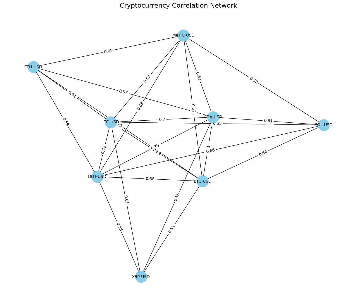
  • Create a Financial Network: Build a graph where nodes represent cryptocurrencies, and edges represent strong correlations.
  • Calculate Graph Laplacian: Analyze the network structure using the Laplacian matrix.
  • Cluster Analysis: Use eigenvalues of the Laplacian to identify independent clusters of cryptocurrencies.
  • Visualize the Network: Plot the graph to reveal clusters and diversification opportunities.

Python Implementation

The following Python code demonstrates how to implement the above steps:

import numpy as np
import pandas as pd
import networkx as nx
import matplotlib.pyplot as plt
from scipy.linalg import eigh
import yfinance as yf

# Fetch Historical Data Using yfinance
def fetch_crypto_data_yfinance(tickers, start_date, end_date):
    data = yf.download(tickers, start=start_date, end=end_date)['Adj Close']
    return data

# Calculate Correlation Matrix
def calculate_correlation_matrix(price_data):
    daily_returns = price_data.pct_change().dropna()
    return daily_returns.corr()

# Create Financial Network
def create_financial_network(correlation_matrix):
    graph = nx.Graph()
    for i, asset1 in enumerate(correlation_matrix.columns):
        for j, asset2 in enumerate(correlation_matrix.columns):
            if i  0.5:
                graph.add_edge(asset1, asset2, weight=correlation_matrix.iloc[i, j])
    return graph

# Calculate Graph Laplacian
def calculate_graph_laplacian(graph):
    return nx.laplacian_matrix(graph).toarray()

# Analyze Clusters Using Eigenvalues
def analyze_clusters(laplacian, crypto_names):
    eigenvalues, _ = eigh(laplacian)
    print("Eigenvalues of the Laplacian:", eigenvalues)
    return np.sum(eigenvalues > 1e-5)

# Visualize the Financial Network
def plot_financial_network(graph):
    pos = nx.spring_layout(graph, seed=42)
    nx.draw(graph, pos, with_labels=True, node_size=800, node_color="skyblue", font_size=10)
    edge_labels = nx.get_edge_attributes(graph, 'weight')
    nx.draw_networkx_edge_labels(graph, pos, edge_labels=edge_labels)
    plt.title("Cryptocurrency Correlation Network")
    plt.show()

# Main Execution
if __name__ == "__main__":
    tickers = ["BTC-USD", "ETH-USD", "SOL-USD", "XRP-USD", "DOT-USD", "ADA-USD", "MATIC-USD", "LTC-USD"]
    start_date = "2023-09-01"
    end_date = "2023-12-01"

    price_data = fetch_crypto_data_yfinance(tickers, start_date, end_date)
    correlation_matrix = calculate_correlation_matrix(price_data)
    financial_network = create_financial_network(correlation_matrix)
    plot_financial_network(financial_network)
    laplacian = calculate_graph_laplacian(financial_network)
    num_clusters = analyze_clusters(laplacian, correlation_matrix.columns)
    print(f"Suggested number of clusters: {num_clusters}")
    

Key Outputs

1. Price Data

Historical adjusted closing prices for cryptocurrencies, retrieved using yfinance.

2. Correlation Matrix

A symmetric matrix showing the relationships between daily returns of cryptocurrencies.

3. Cryptocurrency Network Visualization

A graph where nodes represent cryptocurrencies, and edges represent strong correlations. network

4. Graph Laplacian and Clusters

The Laplacian matrix reveals the structure of the financial network. Eigenvalues identify the number of independent clusters, helping to diversify investments.

Applications in Cryptocurrency Investing

  • Portfolio Diversification: Identify clusters of highly correlated cryptocurrencies to avoid redundancy.
  • Risk Management: Detect systemic risks by analyzing interdependencies.
  • Adaptive Strategies: Dynamically adjust portfolio weights based on evolving clusters.

Conclusion

By applying DDG concepts like graph Laplacians and clustering, cryptocurrency investors can gain valuable insights into market relationships and manage portfolios more effectively. This framework enables better diversification, risk management, and adaptability in volatile crypto markets.